How Convolutional Neural Networks Work

Introduction

Convolutional Neural Networks (CNNs) have revolutionized computer vision, achieving human-level performance in tasks like image classification, object detection, and semantic segmentation. But what makes CNNs so effective at processing visual data? In this post, we'll explore the fundamental mechanisms that power these remarkable architectures.

Unlike traditional fully-connected networks, CNNs exploit the spatial structure of images through three key innovations: local connectivity, parameter sharing, and translation equivariance. These properties allow CNNs to learn hierarchical feature representations efficiently.

CNN Architecture Overview

A typical CNN consists of several types of layers stacked together:

Convolutional Layers: Extract local features using learnable filters
Pooling Layers: Downsample feature maps for spatial invariance
Activation Functions: Introduce non-linearity (ReLU, etc.)
Fully Connected Layers: Perform final classification
Normalization Layers: Stabilize training (BatchNorm, LayerNorm)

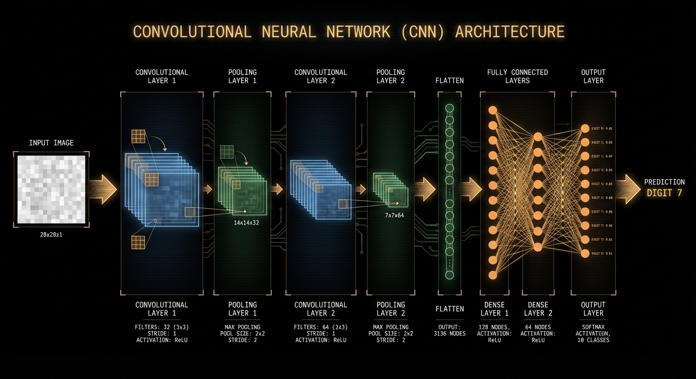
Figure 1: A typical CNN architecture showing the flow from input image through convolutional layers (blue), pooling layers (green), and fully connected layers (orange) to the final output.

The Convolution Operation

What is Convolution?

Think of convolution as a sliding window that scans across an image. At each position, the window (called a filter or kernel) performs a simple calculation: it multiplies its values with the image pixels underneath, then sums everything up to produce a single number.

Example: Imagine a 3×3 filter sliding over a 5×5 image. At each position, we:

Multiply each filter value with the corresponding pixel value
Add all these products together
Store the result in the output
Slide the filter to the next position and repeat

The Math

For a 2D input $X$ and filter $W$ of size $k \times k$, the convolution at position $(i,j)$ is:

(X * W)_{i,j} = \sum_{m=0}^{k-1} \sum_{n=0}^{k-1} X_{i+m, j+n} \cdot W_{m,n}

This formula just says: multiply corresponding elements and sum them up—exactly what we described above!

Figure 2: The convolution operation in action. The filter slides across the input, performing element-wise multiplication and summation at each position.

Key Parameters

Two important settings control how convolution works:

Stride: How many pixels the filter moves each step (stride=1 means move one pixel at a time)
Padding: Adding zeros around the image edges to control output size

Output size formula: For input size $n$, kernel size $k$, stride $s$, and padding $p$:

\text{Output size} = \left\lfloor \frac{n + 2p - k}{s} \right\rfloor + 1

Working with Color Images

RGB images have 3 channels (Red, Green, Blue). The filter also has 3 channels, one for each color. The convolution happens across all channels simultaneously, and the results are summed to produce a single output value. If we want multiple output features, we use multiple filters.

Pooling Operations

After convolution extracts features, pooling helps reduce the size of the data while keeping the important information. Think of it as downsampling or summarizing the feature maps.

Max Pooling

Max pooling divides the input into regions (usually 2×2 squares) and takes the maximum value from each region. This keeps the strongest activations—the most prominent features.

Example: A 2×2 max pooling on a 4×4 image produces a 2×2 output, where each output value is the maximum from its corresponding 2×2 region in the input.

Average Pooling

Average pooling works similarly, but instead of taking the maximum, it computes the average of all values in each region. This provides a smoother, more general representation.

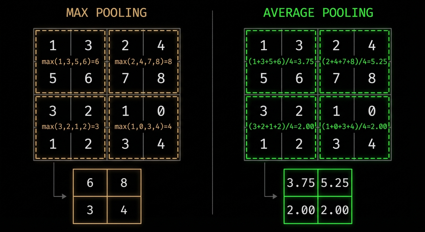
Figure 3: Max pooling (left) selects the highest value from each region, while average pooling (right) computes the mean. Both reduce the spatial dimensions by half.

Why Use Pooling?

Reduces size: Fewer pixels means faster computation and less memory
Position invariance: Small shifts in the input don't change the output much
Broader view: Each layer sees a larger portion of the original image
Prevents overfitting: Reduces the number of parameters to learn

Receptive Field

The receptive field is the area of the original input image that influences a particular neuron's output. Think of it as "how much of the image can this neuron see?"

As we go deeper into the network, each neuron's receptive field grows larger. This is powerful because:

Early layers see small patches (edges, textures) → small receptive field
Middle layers see larger regions (shapes, patterns) → medium receptive field
Deep layers see large areas (whole objects) → large receptive field

Example: In a 5-layer CNN with 3×3 filters:

Layer 1: Sees a 3×3 region of the input
Layer 2: Sees a 5×5 region
Layer 3: Sees a 7×7 region
Layer 4: Sees a 9×9 region
Layer 5: Sees an 11×11 region

This growing receptive field allows the network to build up understanding from simple features to complex objects.

Hierarchical Feature Learning

CNNs learn features in a hierarchical manner:

Early Layers (Low-Level Features)

Edge detectors (horizontal, vertical, diagonal)
Color blobs
Simple textures

Middle Layers (Mid-Level Features)

Corners and contours
Complex textures
Simple shapes (circles, rectangles)

Deep Layers (High-Level Features)

Object parts (eyes, wheels, windows)
Complex patterns
Semantic concepts

This hierarchy emerges naturally from the training process through backpropagation, without explicit programming of what features to detect.

Activation Functions

After convolution, we apply an activation function to introduce non-linearity. Without this, stacking multiple layers would be no better than a single layer!

ReLU (Rectified Linear Unit)

The most popular activation function. ReLU simply outputs the input if it's positive, otherwise outputs zero.
Simple rule: If value > 0, keep it. If value ≤ 0, make it 0.

Why it's great: Fast to compute, helps gradients flow during training, and creates sparse activations.

Leaky ReLU

Similar to ReLU, but instead of completely zeroing negative values, it allows a small negative slope (like 0.01). This prevents neurons from "dying" during training.

GELU (Gaussian Error Linear Unit)

A smoother activation function used in modern architectures like Vision Transformers. It provides better performance for complex tasks but is slightly more expensive to compute.

Batch Normalization

Batch Normalization is a technique that helps neural networks train faster and more stably. The idea is simple: normalize the values in each layer so they have a consistent scale.

How it works: For each batch of data, BatchNorm:

Calculates the mean and variance of the values
Normalizes the values to have mean=0 and variance=1
Applies learnable scaling and shifting to restore representational power

Why Use Batch Normalization?

Faster training: Allows using higher learning rates
More stable: Less sensitive to weight initialization
Regularization effect: Reduces overfitting slightly
Better convergence: Networks train more reliably

Modern CNN Architectures

LeNet-5 (1998)

The pioneering CNN architecture for digit recognition. Structure: Conv → Pool → Conv → Pool → FC → FC

AlexNet (2012)

Breakthrough architecture that won ImageNet 2012. Introduced:

ReLU activation
Dropout for regularization
Data augmentation
GPU training

VGGNet (2014)

Demonstrated that depth matters. Key insights:

Use small 3×3 filters throughout
Stack multiple conv layers before pooling
Deeper networks learn better representations

ResNet (2015)

Introduced residual connections (skip connections) to train very deep networks (up to 152 layers). The key idea: add the input directly to the output, allowing gradients to flow more easily during training.

Why it works: Skip connections solve the vanishing gradient problem, making it possible to train much deeper networks than before.

Inception/GoogLeNet (2014)

Uses parallel convolution paths with different kernel sizes, then combines the results:

1×1 convolutions for dimensionality reduction
Multiple filter sizes in parallel (1×1, 3×3, 5×5)
Efficient computation through bottleneck layers

EfficientNet (2019)

Systematically scales network depth, width, and resolution together for optimal performance. Instead of randomly making networks bigger, EfficientNet finds the best balance between:

Depth: Number of layers
Width: Number of channels per layer
Resolution: Input image size

This achieves state-of-the-art accuracy with fewer parameters than previous models.

Advanced Techniques

Depthwise Separable Convolutions

A clever trick to make CNNs more efficient: instead of one expensive convolution, split it into two cheaper operations:

Depthwise: Apply a separate filter to each input channel
Pointwise: Combine the results with 1×1 convolutions

Result: Up to 9× fewer parameters with similar performance! Used in MobileNet for mobile devices.

Dilated (Atrous) Convolutions

Dilated convolutions add spacing between filter values, allowing them to cover a larger area without adding parameters. Imagine a 3×3 filter that "skips" pixels to effectively see a 5×5 or 7×7 region.

Use case: Semantic segmentation where you need large receptive fields.

Grouped Convolutions

Split the input channels into groups and process each group separately. This reduces computation while maintaining good performance.

Example: Instead of processing 256 channels together, split into 32 groups of 8 channels each.

Practical Considerations

Choosing Hyperparameters

Kernel size: 3×3 is standard, 5×5 or 7×7 for first layer
Stride: 1 for conv layers, 2 for pooling or downsampling
Padding: "same" to preserve spatial dimensions, "valid" to reduce
Number of filters: Powers of 2 (32, 64, 128, 256, 512)

Common Patterns

Conv → BatchNorm → ReLU → Conv → BatchNorm → ReLU → Pool
Double filters when halving spatial dimensions
Use global average pooling instead of FC layers
Add dropout (0.5) before final classification layer

Data Augmentation

Essential for preventing overfitting:

Random crops and flips
Color jittering
Rotation and scaling
Mixup and CutMix

Conclusion

Convolutional Neural Networks have transformed computer vision through their ability to automatically learn hierarchical feature representations. The key mechanisms—convolution, pooling, and non-linear activations—work together to create powerful models that can understand visual data at multiple scales.

Modern architectures like ResNet, EfficientNet, and Vision Transformers build upon these foundations, introducing innovations like skip connections, neural architecture search, and attention mechanisms. Yet the core principles of local connectivity, parameter sharing, and hierarchical learning remain central to their success.

Key Takeaways:

Convolution extracts local features through learnable filters
Pooling provides translation invariance and reduces dimensions
Deep networks learn hierarchical representations automatically
Modern techniques like residual connections enable very deep networks
Proper normalization and regularization are crucial for training