Word2Vec Explained| Omar's Blog

The Problem with Words

Before 2013, computers treated words as atomic symbols. "Apple" and "Orange" were just two different ID numbers, as unrelated as "Apple" and "Car".

We used One-Hot Encoding: a massive vector of zeros with a single '1' at the index of the word.

                    
Apple  = [0, 0, 0, 1, 0, ..., 0]

Orange = [0, 1, 0, 0, 0, ..., 0]

Car    = [0, 0, 0, 0, 0, ..., 1]

The problem? These vectors are orthogonal. The dot product (similarity) between any two words is 0. The computer had no way of knowing that apples and oranges are similar fruits.

Then came Word2Vec (Mikolov et al. at Google), proposing a way to learn Dense Vectors where similar words have similar vectors.

The Core Insight: Distributional Hypothesis

"You shall know a word by the company it keeps." — J.R. Firth (1957)

If two words frequently appear in the same context (surrounded by the same words), they likely mean similar things.

Consider these sentences:

"The dog barked at the mailman."
"The puppy barked at the mailman."

Because "dog" and "puppy" both appear near "barked" and "mailman", the model learns they are semantically related.

1. Generating Training Data (The Sliding Window)

Word2Vec is a self-supervised model. We don't need human labels; we just need raw text. We create a "fake" task to train the model.

We slide a window over the text. The word in the middle is the Target, and the surrounding words are the Context.

Sliding Window Visualization

2. The Architectures: CBOW vs. Skip-gram

The paper proposed two distinct architectures to learn these relationships.

CBOW (Continuous Bag of Words)

Predict the target word from its context

                            
// Given sentence: "The quick brown fox jumps"

Context (Input): ["The", "quick", "fox", "jumps"]

Target (Output): "brown"

// The model averages the context word embeddings

// and predicts the missing middle word

How it works: Take all surrounding words, average their vectors, and use that to predict the center word.

Faster to train
Better for frequent words
Smooths over distributional information

Skip-gram

Predict the context words from the target

                            
// Given sentence: "The quick brown fox jumps"

Target (Input): "brown"

Context (Output): ["The", "quick", "fox", "jumps"]

// The model uses the target word embedding

// to predict each surrounding word

How it works: Take the center word and use it to predict each of the surrounding words independently.

Slower (creates more training pairs)
Better for rare words
Learns finer-grained relationships

Key Difference: CBOW predicts one word from many (many-to-one), while Skip-gram predicts many words from one (one-to-many). Skip-gram creates more training examples because for each target word, it creates a separate training pair with each context word.

3. The "Fake" Task & The Hidden Layer

Here is the secret: We don't actually care about the prediction.

We train a simple neural network (1 hidden layer, no activation function) to perform this prediction task.

Input: One-hot vector of a word (size V).
Hidden Layer: Dense matrix (size V x N). This is the Embedding Matrix!
Output: Softmax probability over all words (size V).

After training, we throw away the output layer. The weights of the hidden layer are the word vectors we wanted all along. If the hidden layer size is 300, each word is now represented by a vector of 300 numbers.

4. The Mathematical Objective: Likelihood Maximization

Now let's understand the math behind Word2Vec. The goal is to learn word vectors that maximize the probability of seeing the actual context words given the target word (Skip-gram) or vice versa (CBOW).

The Likelihood Function

For Skip-gram, given a sequence of words \( w_1, w_2, ..., w_T \), we want to maximize the likelihood of predicting context words from each target word:

\mathcal{L} = \prod_{t=1}^{T} \prod_{-c \leq j \leq c, j \neq 0} P(w_{t+j} | w_t)

Where \(c\) is the context window size

This is a product of probabilities. For each word \(w_t\), we multiply the probabilities of all its context words.

From Products to Sums: The Log-Likelihood

Products are computationally difficult. We apply the logarithm to convert products into sums:

\log \mathcal{L} = \sum_{t=1}^{T} \sum_{-c \leq j \leq c, j \neq 0} \log P(w_{t+j} | w_t)

                    Why logarithm?
                    \(\log(a \times b) = \log(a) + \log(b)\) — converts products to sums
Logarithm is monotonic — maximizing \(\log \mathcal{L}\) is equivalent to maximizing
                            \(\mathcal{L}\)
Prevents numerical underflow (multiplying many small probabilities)

                

The Softmax Probability

How do we calculate \(P(w_O | w_I)\)? Using the softmax function:

P(w_O | w_I) = \frac{\exp(v'_{w_O}{}^T v_{w_I})}{\sum_{w=1}^{W} \exp(v'_w{}^T v_{w_I})}

Where \(v_{w_I}\) is the input embedding and \(v'_{w_O}\) is the output embedding

From Maximization to Minimization: The Loss Function

In practice, optimization algorithms minimize functions, not maximize them. We convert our maximization problem into minimization by adding a negative sign:

\mathcal{J} = -\log \mathcal{L} = -\sum_{t=1}^{T} \sum_{-c \leq j \leq c, j \neq 0} \log P(w_{t+j} | w_t)

The Complete Transformation:

Start: Maximize likelihood (product of probabilities)
Step 1: Take log → product becomes sum
Step 2: Add negative sign → maximization becomes minimization
Result: Loss function \(\mathcal{J}\) that we can minimize with gradient descent!

Substituting the softmax probability:

\mathcal{J} = -\sum_{t=1}^{T} \sum_{-c \leq j \leq c, j \neq 0} \left[ v'_{w_{t+j}}{}^T v_{w_t} - \log \sum_{w=1}^{W} \exp(v'_w{}^T v_{w_t}) \right]

This is the negative log-likelihood loss, also known as cross-entropy loss. The problem? That summation over all \(W\) words in the vocabulary is extremely expensive!

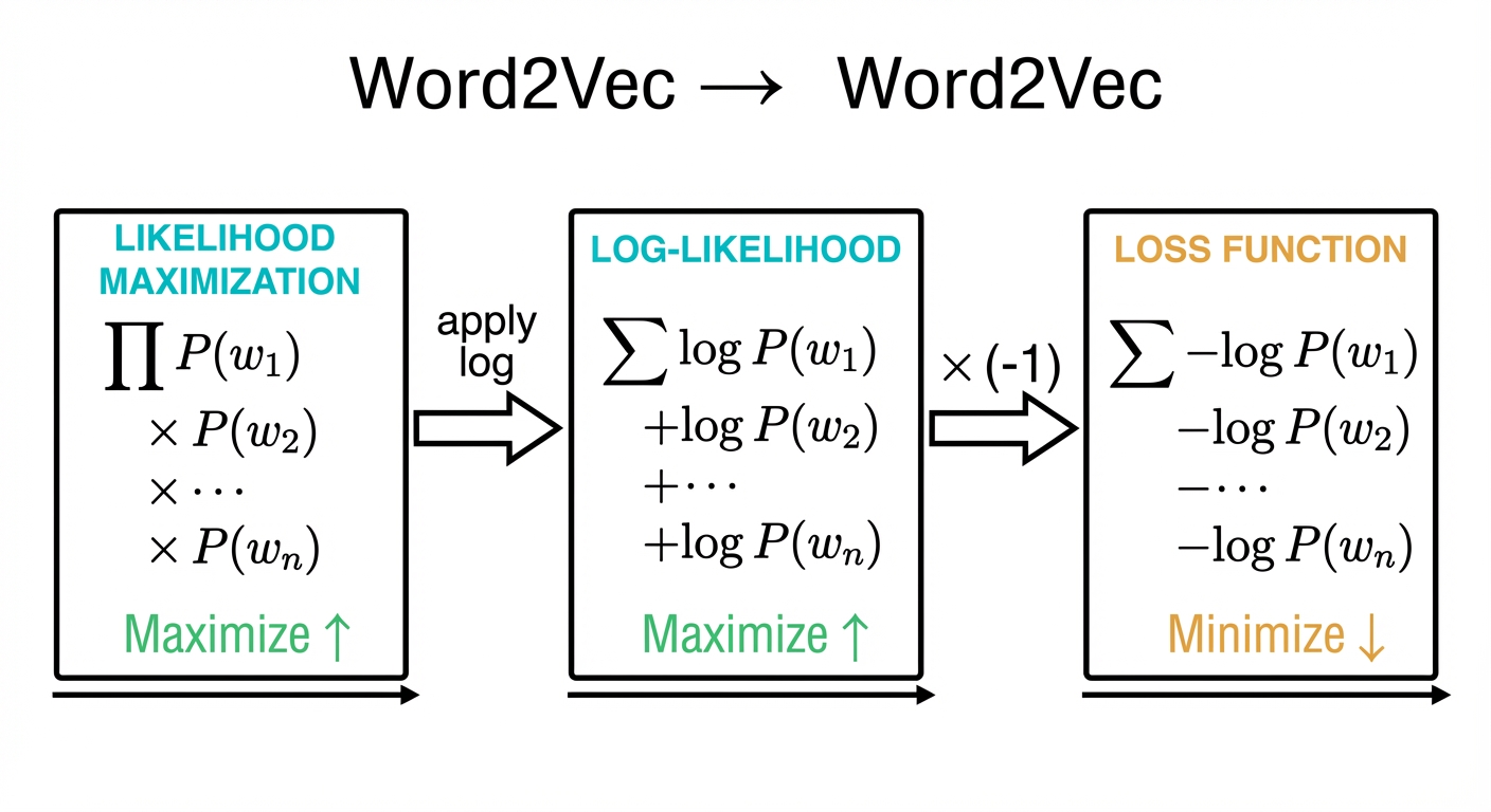
Visual summary: From likelihood maximization to loss minimization

5. Optimization: Negative Sampling

The Computational Problem

Calculating the Softmax over a vocabulary of 100,000+ words for every single training example is incredibly slow. The denominator requires summing exponentials for every word.

P(w_O | w_I) = \frac{\exp(v'_{w_O}{}^T v_{w_I})}{\sum_{w=1}^W \exp(v'_w{}^T v_{w_I})}

For a vocabulary of 100,000 words, we need to compute 100,000 dot products and exponentials for every single training example. With billions of training examples, this becomes computationally infeasible.

The Negative Sampling Solution

Key Insight: Instead of trying to predict the exact probability distribution over all words, we can frame it as a binary classification problem: "Is this word pair (target, context) from the real data or not?"

For each positive example (actual context word), we sample a few (typically 5-20) "negative" examples (random words that aren't in the context). We then train the model to:

Output high probability (close to 1) for the positive example
Output low probability (close to 0) for the negative examples

The Negative Sampling Objective

Instead of the full softmax, we use the sigmoid function for binary classification. The formal objective function defined in the paper is:

J = -\log \sigma(v'_{w_c}{}^T v_{w_t}) - \sum_{i=1}^{k} \mathbb{E}_{w_i \sim P_n(w)} \left[ \log \sigma(-v'_{w_i}{}^T v_{w_t}) \right]

In practice, for a single training step with \(k\) specific negative samples, this simplifies to:

J = - \underbrace{\log \sigma(v'_{w_c}{}^T v_{w_t})}_{\text{Positive Pair}} - \sum_{i=1}^{k} \underbrace{\log \sigma(-v'_{w_{neg_i}}{}^T v_{w_t})}_{\text{Negative Samples}}

🎯 The Sigmoid Strategy: Both Aim for 1, Different Paths

The model tries to make both positive and negative pairs achieve a sigmoid output close to 1, but through different mechanisms:

🔵 Positive Pairs

\( v' \cdot v \) → large positive

Goal: \( \sigma(v' \cdot v) \approx 1 \)
Strategy: Align vectors (same direction)

🔴 Negative Pairs

\( v'_{neg} \cdot v \) → large negative

Goal: \( \sigma(-v'_{neg} \cdot v) \approx 1 \)
Strategy: Reverse vectors (opposite direction)

Key Insight: The negative sign inside \( \sigma(-v'_{neg} \cdot v) \) flips the dot product. So when \( v'_{neg} \cdot v \) is large and negative (vectors pointing opposite), \( -v'_{neg} \cdot v \) becomes large and positive, making \( \sigma(-v'_{neg} \cdot v) \approx 1 \). Both formulations reward the model when sigmoid outputs 1, but they achieve this through different vector geometries.

Geometric Result: By minimizing \(J\) over billions of examples, the model learns a vector space where semantically similar words (which appear in similar contexts) are clustered together through alignment, while unrelated words are pushed apart through opposition.

Deep Dive: Deconstructing the Objective Function

Let's break down exactly why the equation looks the way it does, step by step.

A. What We Want to Do

We want to predict whether a word pair is real (1) or fake (0).
We want dot products of positive pairs → large positive.
We want dot products of negative pairs → large negative.
We want a loss function that rewards correct predictions and punishes wrong predictions.
We want a loss that uses sigmoid(probability) and is minimized, not maximized.

B. Why is there a "− INSIDE log"? (sigmoid(-dot))

For negative samples, the target probability is 0.
Sigmoid(s) = probability of label=1.
Probability of label=0 = 1 - sigmoid(s) = sigmoid(-s).
Therefore, we use sigmoid(-dot) for negative samples. This forces the dot product to become negative.

C. Why is there a "− OUTSIDE log"? (−log(p))

log(probability) is always negative (since p < 1). We must flip the sign.
We want loss ≥ 0 → need the minus.
Maximizing log(p) is equivalent to minimizing -log(p).
Standard binary cross-entropy has a minus sign. Without it, gradients would push in the wrong direction.

D. Cross-Entropy Derivation Structure

Start from information: \( I(x) = -\log(x) \).
Entropy = expected information = \( \sum p \log(1/p) \).
Cross entropy = \( \sum p(x) \cdot [-\log q(x)] \).
Binary case yields: \( -[ t \log y + (1-t) \log(1-y) ] \).
Plug \( y = \text{sigmoid}(\text{dot}) \).

E. Final Word2Vec Loss Forms

Positive sample loss = \( -\log(\text{sigmoid}(\text{dot})) \).
Negative sample loss = \( -\log(\text{sigmoid}(-\text{dot})) \).
Full loss = sum over all positives + negatives.

F. Optimization Goals

Minimize positive loss → increase dot product.
Minimize negative loss → decrease dot product.
Dot product increases/decreases via gradient descent updates.

Where \(\sigma(x) = \frac{1}{1 + e^{-x}}\) is the sigmoid function and \(k\) is the number of negative samples (usually 5-20).

                    
// Example: Target word = "fox", Context word = "quick"

Positive pair: ("fox", "quick") → Train to output 1

Negative samples (k=5):

  ("fox", "democracy") → Train to output 0

  ("fox", "pizza")     → Train to output 0

  ("fox", "algorithm") → Train to output 0

  ("fox", "ocean")     → Train to output 0

  ("fox", "guitar")    → Train to output 0

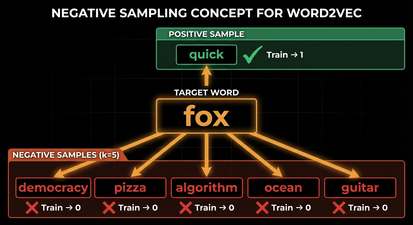
Negative sampling: 1 positive example + k negative examples

How to Sample Negative Examples?

We don't sample uniformly! The paper uses a unigram distribution raised to the 3/4 power:

P(w_i) = \frac{f(w_i)^{3/4}}{\sum_{j=1}^{W} f(w_j)^{3/4}}

Where \(f(w_i)\) is the frequency of word \(w_i\) in the corpus

Why the 3/4 power?

Uniform sampling (\(P(w) = 1/W\)) gives too many rare words
Frequency-based sampling (\(P(w) \propto f(w)\)) gives too many common words like "the", "a"
The 3/4 power is a sweet spot that slightly favors rare words without overwhelming the model
Example: If "the" appears 1000× more than "giraffe", with 3/4 power it's only sampled ~178× more often

Computational Savings

Instead of computing probabilities for 100,000 words, we now only compute for 1 positive + 5-20 negatives = 6-21 words. This is a ~5000× speedup!

                    Negative Sampling vs. Full Softmax:

                    Full Softmax: O(W) complexity per training example (W = vocabulary
                            size)
                        
Negative Sampling: O(k) complexity per training example (k = 5-20)
Result: Training becomes feasible on large corpora with billions of
                            words!

6. The Result: Semantic Arithmetic

The most famous result from the paper was the emergence of linear substructures. The model learned relationships that allowed for vector arithmetic.

King - Man + Woman ≈ Queen

If you take the vector for King, subtract the "maleness" vector (Man), and add the "femaleness" vector (Woman), the closest resulting vector in the space is Queen.

Other examples found:

Paris - France + Italy ≈ Rome (Capital cities)
Bigger - Big + Small ≈ Smaller (Adjective scaling)
Einstein - Scientist + Painter ≈ Picasso

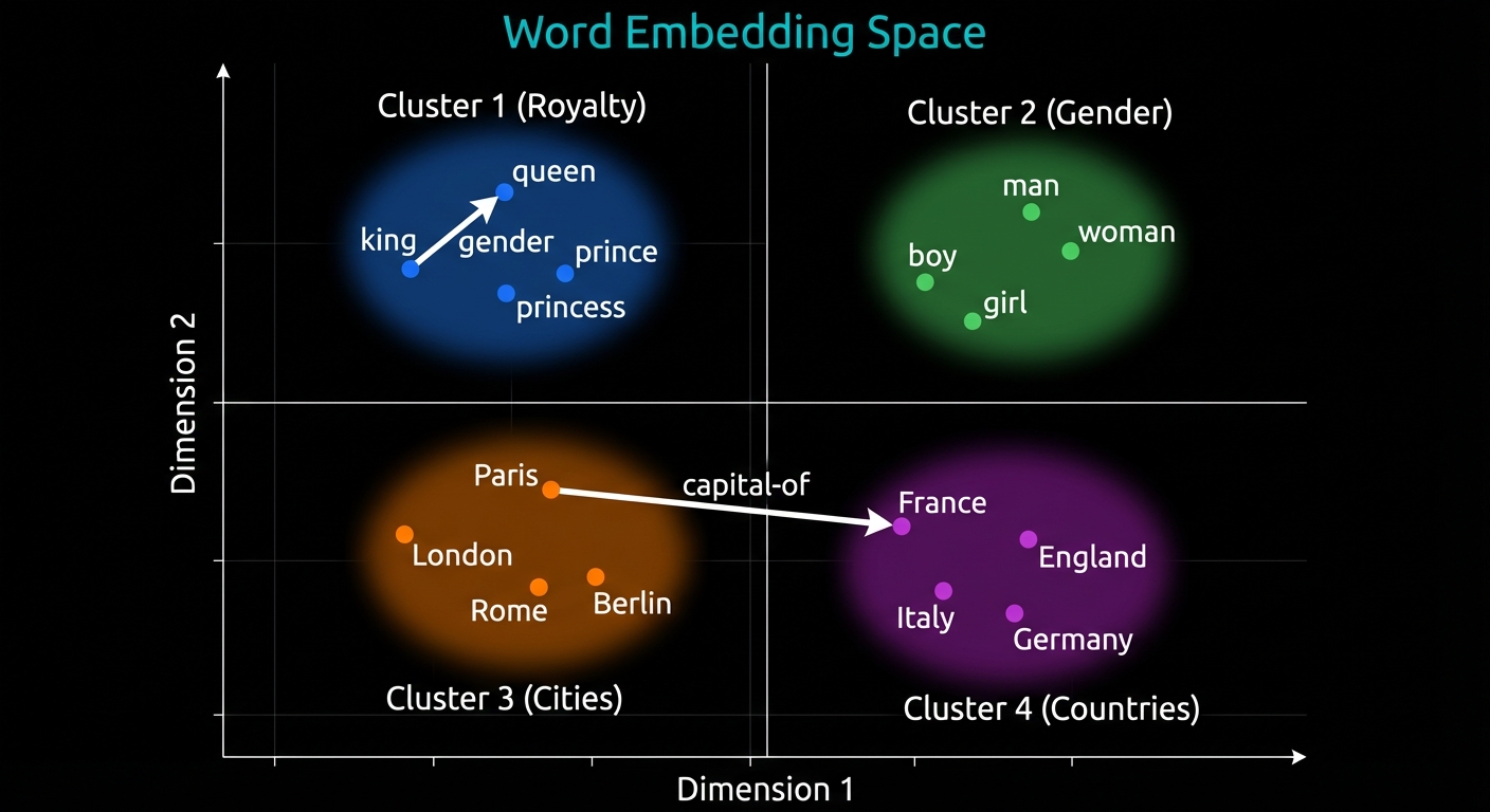
2D projection of word embeddings showing semantic clusters and relationships

7. Training Details & Hyperparameters

Key Hyperparameters

The Word2Vec paper provides specific recommendations for training:

Vector Dimensionality

Typical: 100-300 dimensions
Small datasets: 50-100 dims
Large datasets: 300-500 dims
Higher dimensions capture more nuance but risk overfitting

Context Window Size

Skip-gram: 5-10 words
CBOW: 5-10 words
Larger windows capture topic similarity
Smaller windows capture syntactic relationships

Negative Samples

Small datasets: 5-20 samples
Large datasets: 2-5 samples
More negatives = better quality but slower
Paper recommends 5-20 for best results

Learning Rate & Epochs

Initial LR: 0.025
Decay: Linear to 0.0001
Epochs: 5-15 passes
Use SGD (Stochastic Gradient Descent)

Subsampling Frequent Words

Common words like "the", "a", "in" appear so frequently that they provide little information. The paper uses subsampling to randomly discard them during training:

P(\text{discard } w_i) = 1 - \sqrt{\frac{t}{f(w_i)}}

Where \(t\) is a threshold (typically \(10^{-5}\)) and \(f(w_i)\) is the word frequency

Effect of Subsampling:

Words with frequency > threshold are randomly discarded
"the" (very frequent) might be discarded 99% of the time
"giraffe" (rare) is almost never discarded
Speeds up training 2-10× while improving quality

Implementation

You can find my full implementation of the paper from scratch on GitHub: word2vec-implementation

Conclusion

Word2Vec was a pivotal moment in AI. It showed that simple neural networks, given enough data, could capture complex human concepts like analogy and semantic relationship without being explicitly taught grammar or logic.

Why Word2Vec Matters

Simplicity: Just a 2-layer neural network with no complex architecture
Efficiency: Negative sampling made training on billions of words feasible
Generality: Works across languages, domains, and even non-text data
Foundation: Paved the way for modern NLP (BERT, GPT, etc.)

Modern Context

While we now use Transformers and Contextual Embeddings (like BERT and GPT), Word2Vec remains:

Widely used for lightweight applications and small datasets
Educational — the best introduction to embeddings and representation learning
Still relevant in production systems where speed matters more than perfect accuracy

                    Key Takeaways:
                    Words are represented as dense vectors in continuous space
Similar words have similar vectors (measured by cosine similarity)
The model learns by predicting context from target (Skip-gram) or vice versa (CBOW)
Negative sampling makes training computationally feasible
The resulting embeddings capture semantic and syntactic relationships

                