Information Theory Part 3: KL Divergence

The Story So Far

In Part 1, we defined Entropy \( H(P) \): the minimum bits needed to encode the truth.

In Part 2, we defined Cross-Entropy \( H(P, Q) \): the bits we actually used because we optimized for the wrong distribution \( Q \).

Now, we simply subtract the two.

Defining KL Divergence

Kullback-Leibler (KL) Divergence is just the difference between the Cross-Entropy and the Entropy. It measures the extra bits we wasted.

D_{KL}(P || Q) = \underbrace{H(P, Q)}_{\text{Bits Used}} - \underbrace{H(P)}_{\text{Optimal Bits}}

If we expand the terms, we get the famous formula:

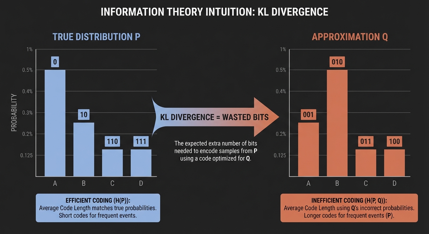
D_{KL}(P || Q) = \sum_{x} P(x) \log \left( \frac{P(x)}{Q(x)} \right)

Figure 1: KL Divergence represents the "wasted bits" (inefficiency) when using approximation Q.

Why isn't it a Distance?

We often call KL Divergence a "distance" between distributions, but it lacks a key property: Symmetry.

D_{KL}(P || Q) \neq D_{KL}(Q || P)

Going from A to B is not the same as going from B to A. This matters a lot in Machine Learning.

Forward KL: \( D_{KL}(P || Q) \)

"Mean Seeking"

Used in Supervised Learning. We want our model \( Q \) to cover all the data in \( P \). If \( P(x) > 0 \), \( Q(x) \) must be \( > 0 \).

Reverse KL: \( D_{KL}(Q || P) \)

"Mode Seeking"

Used in Reinforcement Learning and Variational Inference. The model \( Q \) tries to fit just one part of \( P \) really well, ignoring the rest.

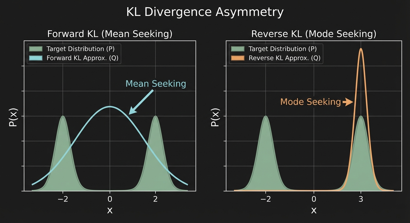
Figure 2: Forward KL (left) stretches to cover everything. Reverse KL (right) focuses on the peak.

Conclusion

We've completed our journey through Information Theory:

Entropy: The inherent uncertainty of the universe.
Cross-Entropy: The practical cost of our imperfect models.
KL Divergence: The measure of our inefficiency.

These three concepts form the backbone of modern AI. Every time you train a classifier, you are minimizing Cross-Entropy. Every time you train a VAE, you are minimizing KL Divergence.