Maximum Likelihood Estimation Explained

What is Maximum Likelihood Estimation?

Maximum Likelihood Estimation (MLE) is one of the most fundamental concepts in statistics and machine learning. It answers a simple question: Given some observed data, what parameters of our model make this data most likely?

MLE is everywhere in machine learning:

Training linear regression models
Fitting probability distributions
Learning neural network weights
Estimating parameters in statistical models

Definition: Maximum Likelihood Estimation is a method of estimating the parameters of a probability distribution by maximizing the likelihood function, which measures how well the model explains the observed data.

The Core Intuition

Imagine you have a coin, and you flip it 10 times. You get 7 heads and 3 tails. What's the probability that this coin lands on heads?

Your intuition probably says: "Well, 7 out of 10 flips were heads, so the probability is probably around 0.7 (70%)." That intuition is exactly MLE!

Example: Coin Flip

Observed data: 7 heads, 3 tails

Question: What value of \( p \) (probability of heads) makes this observation most likely?

MLE answer: \( \hat{p} = \frac{7}{10} = 0.7 \)

MLE formalizes this intuition mathematically. It finds the parameter values that maximize the probability (likelihood) of observing the data we actually observed.

Mathematical Framework

Likelihood Function

Given observed data \( X = \{x_1, x_2, \ldots, x_n\} \) and a model with parameters \( \theta \), the likelihood function is:

\mathcal{L}(\theta | X) = P(X | \theta) = \prod_{i=1}^{n} P(x_i | \theta)

This reads as: "The likelihood of parameters \( \theta \) given data \( X \) equals the probability of observing \( X \) if \( \theta \) were the true parameters."

                    Key Insight: We treat the data as fixed (we observed it) and the parameters as
                    variable (we're trying to find them). This is the opposite of probability, where parameters are
                    fixed and data varies.
                

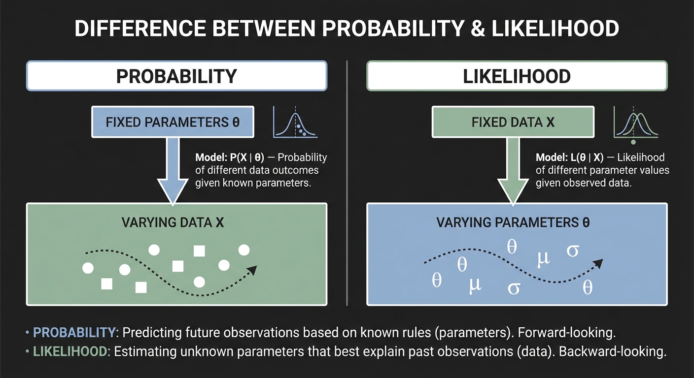
Figure 1: The key difference between probability and likelihood

Log-Likelihood

Products are hard to work with mathematically. Since logarithm is monotonically increasing, maximizing \( \mathcal{L}(\theta) \) is equivalent to maximizing \( \log \mathcal{L}(\theta) \):

\ell(\theta) = \log \mathcal{L}(\theta) = \sum_{i=1}^{n} \log P(x_i | \theta)

The log-likelihood turns products into sums, which are much easier to differentiate and optimize.

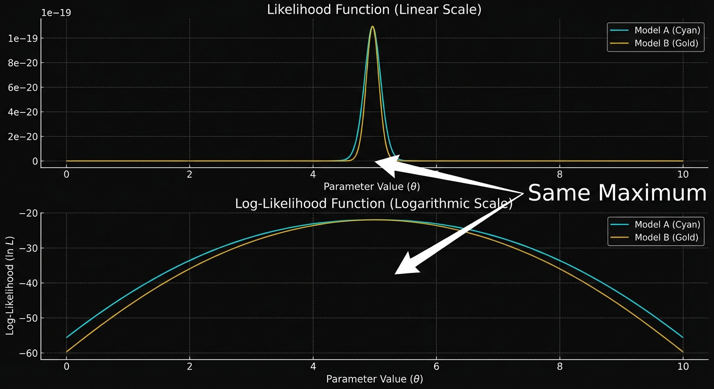
Figure 2: Why we use log-likelihood - same maximum, easier optimization

Finding the Maximum

To find the MLE, we take the derivative of the log-likelihood with respect to \( \theta \), set it to zero, and solve:

\frac{\partial \ell(\theta)}{\partial \theta} = 0

This gives us the critical points. We verify it's a maximum (not minimum) by checking the second derivative is negative.

Example 1: Bernoulli Distribution (Coin Flips)

Let's formalize the coin flip example mathematically.

Step 1: Define the Model

Each coin flip follows a Bernoulli distribution with parameter \( p \) (probability of heads):

P(x_i | p) = p^{x_i} (1-p)^{1-x_i}

where \( x_i = 1 \) for heads, \( x_i = 0 \) for tails.

Step 2: Write the Likelihood

For \( n \) independent flips with \( k \) heads:

\mathcal{L}(p) = \prod_{i=1}^{n} p^{x_i} (1-p)^{1-x_i} = p^k (1-p)^{n-k}

Step 3: Take the Log-Likelihood

\ell(p) = \log \mathcal{L}(p) = k \log p + (n-k) \log(1-p)

Step 4: Differentiate and Set to Zero

\frac{\partial \ell}{\partial p} = \frac{k}{p} - \frac{n-k}{1-p} = 0

Step 5: Solve for \( p \)

\begin{align} \frac{k}{p} &= \frac{n-k}{1-p} \\ k(1-p) &= p(n-k) \\ k - kp &= np - kp \\ k &= np \\ \hat{p} &= \frac{k}{n} \end{align}

Result

The MLE for the Bernoulli parameter is simply the proportion of successes:

\hat{p}_{\text{MLE}} = \frac{\text{number of heads}}{\text{total flips}} = \frac{k}{n}

For our example with 7 heads out of 10 flips: \( \hat{p} = \frac{7}{10} = 0.7 \)

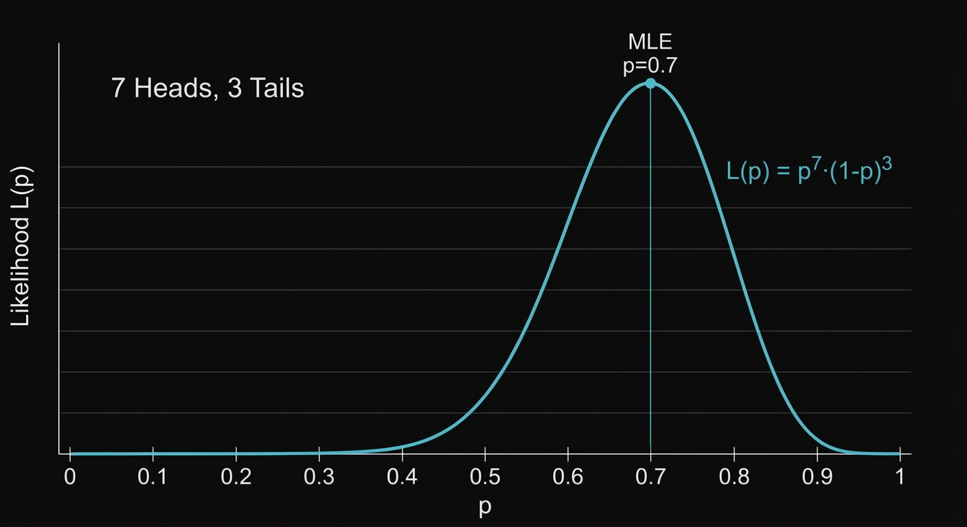
Figure 3: Likelihood function for coin flip example - peaks at p=0.7

Example 2: Normal Distribution

A more complex example: estimating the mean \( \mu \) and variance \( \sigma^2 \) of a normal distribution from data.

Step 1: Normal Distribution PDF

P(x_i | \mu, \sigma^2) = \frac{1}{\sqrt{2\pi\sigma^2}} \exp\left(-\frac{(x_i - \mu)^2}{2\sigma^2}\right)

Step 2: Likelihood for \( n \) Observations

\mathcal{L}(\mu, \sigma^2) = \prod_{i=1}^{n} \frac{1}{\sqrt{2\pi\sigma^2}} \exp\left(-\frac{(x_i - \mu)^2}{2\sigma^2}\right)

Step 3: Log-Likelihood

\begin{align} \ell(\mu, \sigma^2) &= \sum_{i=1}^{n} \log P(x_i | \mu, \sigma^2) \\ &= -\frac{n}{2}\log(2\pi) - \frac{n}{2}\log(\sigma^2) - \frac{1}{2\sigma^2}\sum_{i=1}^{n}(x_i - \mu)^2 \end{align}

Step 4: Maximize with Respect to \( \mu \)

Take derivative with respect to \( \mu \) and set to zero:

\frac{\partial \ell}{\partial \mu} = \frac{1}{\sigma^2}\sum_{i=1}^{n}(x_i - \mu) = 0

Solving:

\hat{\mu}_{\text{MLE}} = \frac{1}{n}\sum_{i=1}^{n} x_i = \bar{x}

Step 5: Maximize with Respect to \( \sigma^2 \)

Take derivative with respect to \( \sigma^2 \) and set to zero:

\frac{\partial \ell}{\partial \sigma^2} = -\frac{n}{2\sigma^2} + \frac{1}{2\sigma^4}\sum_{i=1}^{n}(x_i - \mu)^2 = 0

Solving:

\hat{\sigma}^2_{\text{MLE}} = \frac{1}{n}\sum_{i=1}^{n}(x_i - \bar{x})^2

Result

The MLE estimates for a normal distribution are:

Mean: Sample mean \( \hat{\mu} = \bar{x} \)
Variance: Sample variance \( \hat{\sigma}^2 = \frac{1}{n}\sum(x_i - \bar{x})^2 \)

Note: The MLE for variance is biased (uses \( n \) instead of \( n-1 \)). The unbiased estimator uses \( n-1 \).

Connection to Linear Regression

Linear regression can be derived using MLE! This shows how fundamental MLE is to machine learning.

The Setup

Assume our data follows:

y_i = \mathbf{w}^T \mathbf{x}_i + \epsilon_i, \quad \epsilon_i \sim \mathcal{N}(0, \sigma^2)

This means \( y_i \) is normally distributed around the prediction:

y_i | \mathbf{x}_i, \mathbf{w} \sim \mathcal{N}(\mathbf{w}^T \mathbf{x}_i, \sigma^2)

Likelihood

\mathcal{L}(\mathbf{w}) = \prod_{i=1}^{n} \frac{1}{\sqrt{2\pi\sigma^2}} \exp\left(-\frac{(y_i - \mathbf{w}^T\mathbf{x}_i)^2}{2\sigma^2}\right)

Log-Likelihood

\ell(\mathbf{w}) = -\frac{n}{2}\log(2\pi\sigma^2) - \frac{1}{2\sigma^2}\sum_{i=1}^{n}(y_i - \mathbf{w}^T\mathbf{x}_i)^2

Maximizing

Maximizing the log-likelihood is equivalent to minimizing:

\sum_{i=1}^{n}(y_i - \mathbf{w}^T\mathbf{x}_i)^2

                    Key Result: Maximizing the likelihood under Gaussian noise is exactly equivalent to
                    minimizing the squared error (least squares)! This is why we use MSE loss in regression.
                

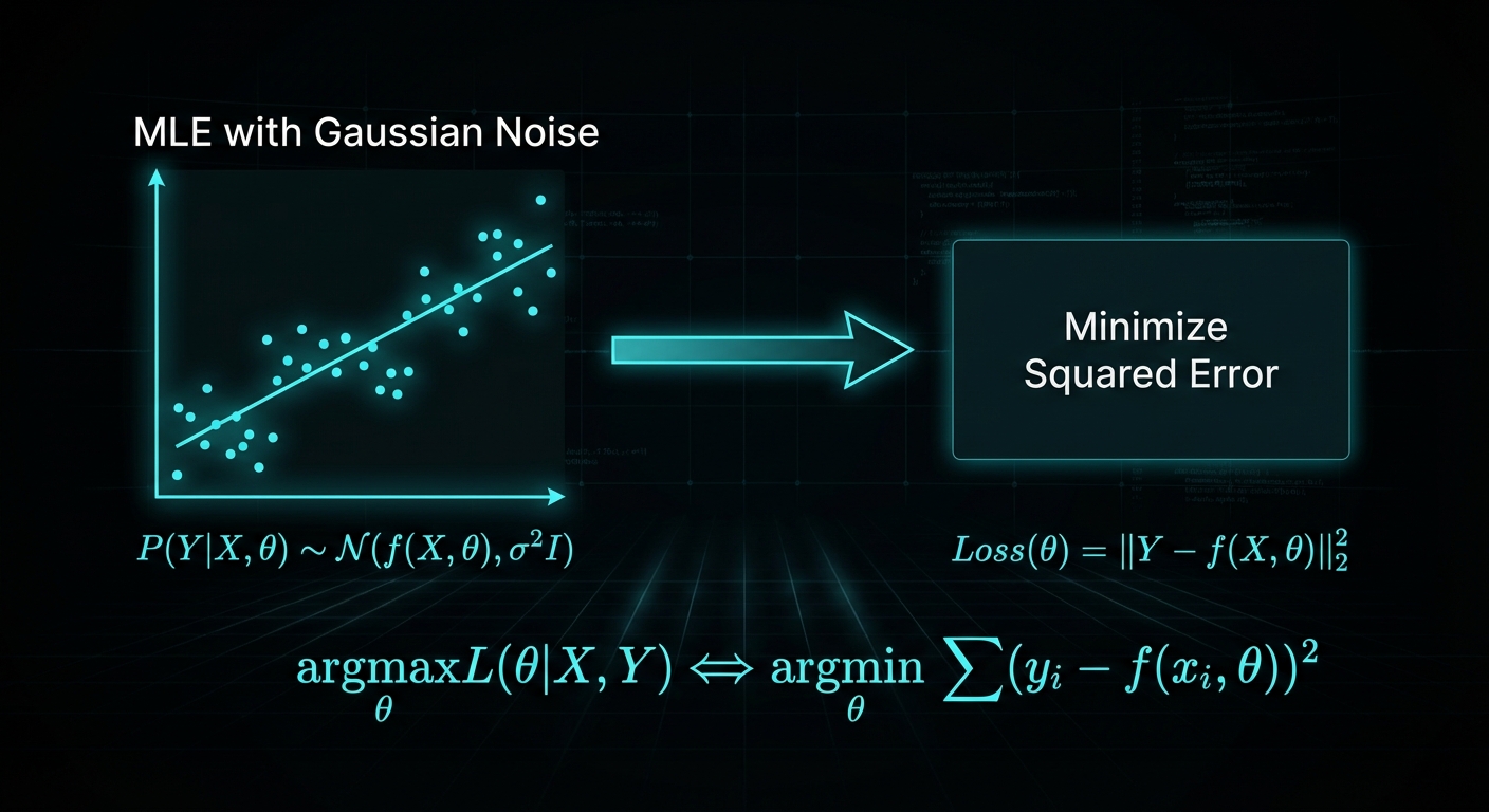
Figure 4: How MLE under Gaussian noise leads to least squares regression