Optimization Theory for Deep Learning Losses

Introduction

At the heart of deep learning lies a deceptively simple idea: adjust the parameters of a neural network to minimize a loss function. Yet beneath this simplicity lies a rich mathematical landscape involving non-convex optimization, stochastic gradients, and complex convergence dynamics. In this post, we'll explore the theoretical foundations that make modern deep learning possible.

The Optimization Problem

Training a neural network can be formulated as solving the following optimization problem:

\begin{aligned} \min_{\theta \in \mathbb{R}^d} \quad & L(\theta) = \frac{1}{n} \sum_{i=1}^{n} \ell(f(x_i; \theta), y_i) \end{aligned}

where:

$\theta \in \mathbb{R}^d$: model parameters (weights and biases)
$f(x; \theta)$: neural network function
$\ell$: loss function (e.g., cross-entropy, MSE)
$(x_i, y_i)$: training data pairs
$n$: number of training examples

This formulation, while elegant, hides several challenges. The loss landscape $L(\theta)$ is typically non-convex, high-dimensional, and contains numerous local minima, saddle points, and flat regions.

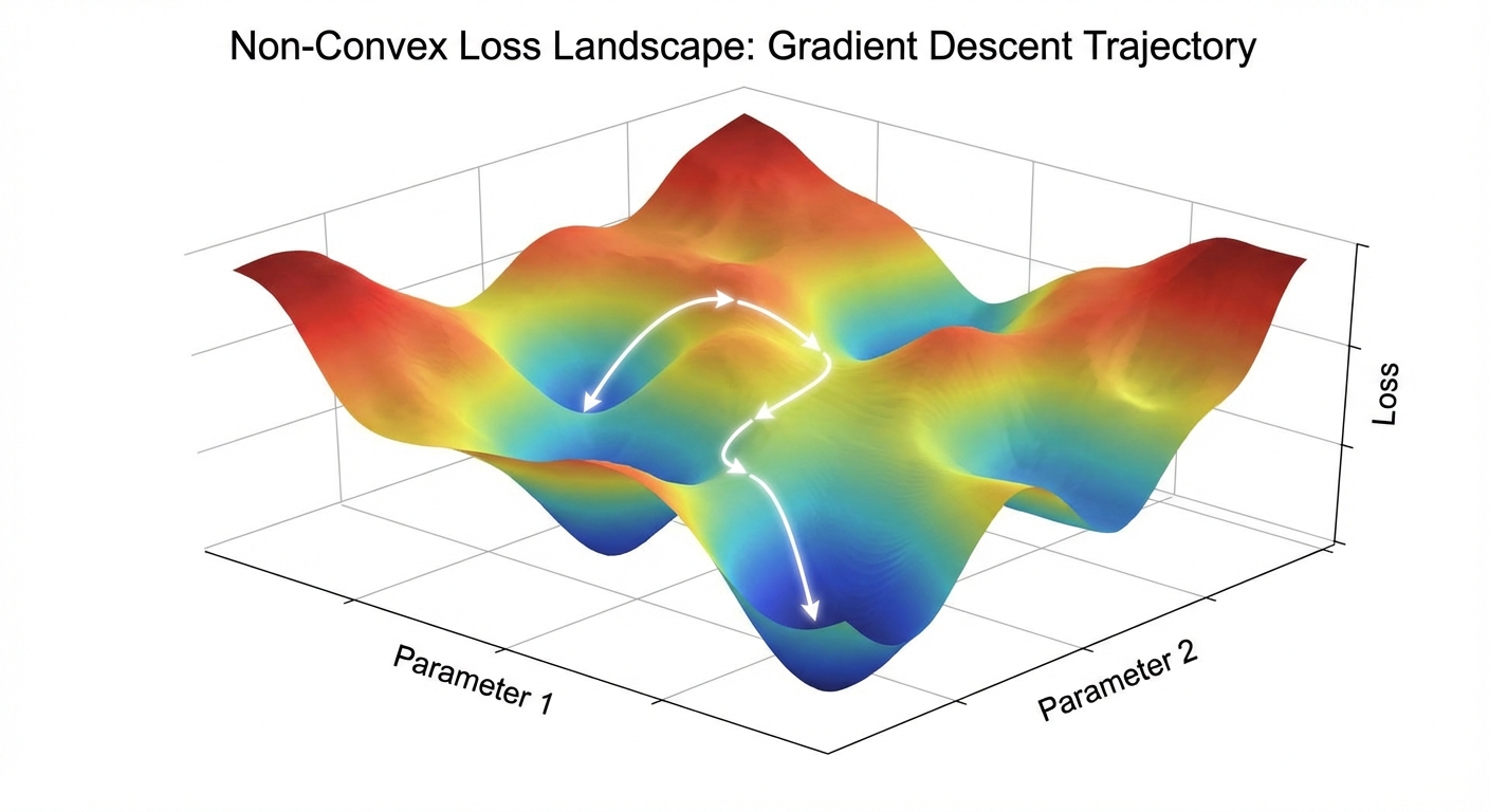
Figure 1: 3D visualization of a non-convex loss landscape showing local minima, saddle points, and a gradient descent trajectory navigating toward the global minimum.

Gradient Descent: The Engine of Learning

The Intuition: A Hiker in the Fog

Imagine you are a hiker stuck on a mountain at night. It's pitch black (or foggy), so you can't see the bottom of the valley (the minimum loss).

What do you do? You feel the ground with your feet.

Feel the slope: You check which direction goes down the steepest.
Take a step: You take a small step in that direction.
Repeat: You keep doing this until the ground becomes flat (you reached the bottom).

This is exactly what Gradient Descent does. The "mountain" is the Loss Function, and the "step" is the parameter update.

The Algorithm

Mathematically, we update our parameters $\theta$ (weights) using the gradient $\nabla L(\theta)$:

\theta_{\text{new}} = \theta_{\text{old}} - \eta \cdot \nabla L(\theta_{\text{old}})

Let's break it down:

$\theta_{\text{old}}$: Where we are now.
$\nabla L(\theta_{\text{old}})$: The direction of steepest ascent (uphill).
$-\nabla L(\theta_{\text{old}})$: The direction of steepest descent (downhill).
$\eta$ (Eta): The Learning Rate. This determines how big of a step we take.

The Importance of Learning Rate ($\eta$)

The learning rate is the most important hyperparameter.

Too Small: You will take tiny baby steps. It will take forever to reach the bottom.
Too Big: You might jump across the valley and land on the other side (overshooting), or even climb up higher!
Just Right: You descend smoothly and efficiently.

Stochastic Gradient Descent (SGD)

In standard Gradient Descent, we calculate the slope using all the data points. If you have 1 million images, this is incredibly slow.

Stochastic Gradient Descent (SGD) is a shortcut. Instead of looking at the whole mountain, we just look at a small "batch" of data (e.g., 32 images) to estimate the slope.

It's a bit noisy—like stumbling around slightly—but it's much faster and, surprisingly, the noise often helps us escape bad spots (local minima).

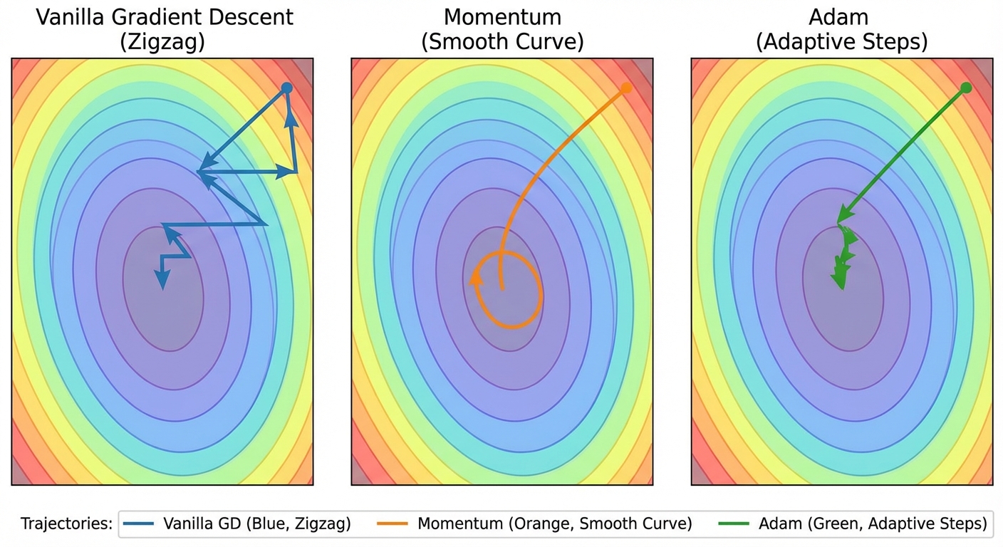
Figure 2: Comparison of optimization trajectories. Vanilla SGD (blue) can be noisy, while Momentum (orange) and Adam (green) smooth out the path.

Advanced Optimization Algorithms

Momentum: The Heavy Ball

Imagine a ball rolling down a hill. It doesn't just stop the moment the slope gets flat; it has momentum.

In optimization, we do the same thing. Instead of just following the current gradient, we keep a "velocity" vector. If we are moving in the same direction for a while, we speed up. If the gradient changes direction (like in a zigzag valley), the momentum keeps us moving forward, smoothing out the path.

Adam: Adaptive Learning Rates

Adam (Adaptive Moment Estimation) is the most popular optimizer today.

The key idea is simple: Not all parameters need the same learning rate.

Some features are rare (sparse), so we want to take big steps when we see them.
Some features are common, so we want to be careful and take small steps.

Adam keeps track of the "history" of gradients for each parameter individually and adjusts their learning rates automatically. This makes it much easier to tune than standard SGD.

Conclusion

Optimization in deep learning is about navigating a complex landscape to find a good solution.

While SGD is the foundation, modern optimizers like Adam and Momentum add clever tricks to make training faster and more stable.

Key Takeaway: For most new projects, start with Adam (learning rate around 0.001). If you need absolute state-of-the-art performance (like in research papers), you might switch to SGD with Momentum later, but Adam is the best "default" choice.